
確率的最適化アルゴリズムの実装と比較:遺伝的アルゴリズムと勾配降下法
はじめに
実務で出会う最適化問題の多くは非凸で、勾配に沿って下るだけでは途中の局所解に捕まります。この対処として、勾配を使わず解の集団で探索する方法が古くから使われてきました。性質の異なる2つの手法、勾配降下法(Gradient Descent: GD)と遺伝的アルゴリズム(Genetic Algorithm: GA)を同じ条件で実装し、局所解の多い4つのベンチマーク関数で解の質・成功率・計算時間を比べました。先に結果を言うと、局所解が多い関数ではGAが最も良い解に届き、その代わり計算時間は勾配法の4倍前後かかります。
対象読者:
- 最適化アルゴリズムの基礎を理解したい方
- 勾配降下法と遺伝的アルゴリズムの違いを知りたい方
- Pythonを用いた最適化問題の解法に興味がある方
記事のポイント:
- 勾配降下法と遺伝的アルゴリズムの原理と実装を示します
- 4つのベンチマーク関数で、解の質・成功率・計算時間を比較します
- 実験結果に基づいて、どちらをどんな問題で選ぶかを考察します
比較する手法:勾配法と遺伝的アルゴリズム
勾配降下法(Gradient Descent: GD)
勾配降下法は、目的関数の勾配(偏微分)を利用して、関数値が減少する方向に解を更新していく手法です。更新式は以下の通りです。
ここで、 は学習率、 は点 における目的関数 の勾配です。
局所的には効率よく解を改善できますが、出発点しだいで局所的最適解に落ち着いてしまい、そこから抜け出す仕組みを持ちません。
モーメンタム付き勾配降下法(Momentum GD)
モーメンタム付き勾配降下法は、通常の勾配降下法に「慣性」を導入し、過去の更新方向の情報を利用します。
ここで、 はモーメンタム係数、 は時刻 における速度ベクトルです。
遺伝的アルゴリズム(Genetic Algorithm: GA)
遺伝的アルゴリズムは、生物の進化を模した最適化手法です。複数の解候補(個体)からなる集団を維持し、適合度(目的関数値)の良い個体を次世代に残す選択(selection)、選ばれた個体同士の成分を混ぜて新しい個体を作る交叉(crossover)、低い確率で成分をランダムに置き換える突然変異(mutation)の3つの操作を繰り返します。
集団で広く探すため局所的最適解に捕まりにくい反面、1世代ごとに集団全体を評価するので、計算コストは勾配法より大きくなります。
実験設計
テスト関数
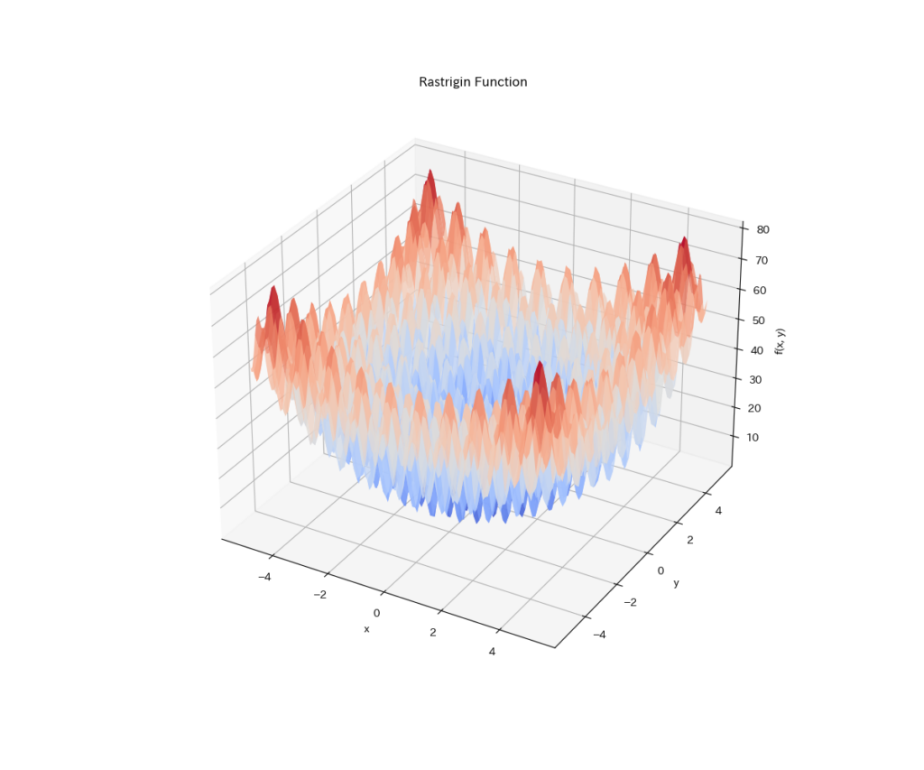
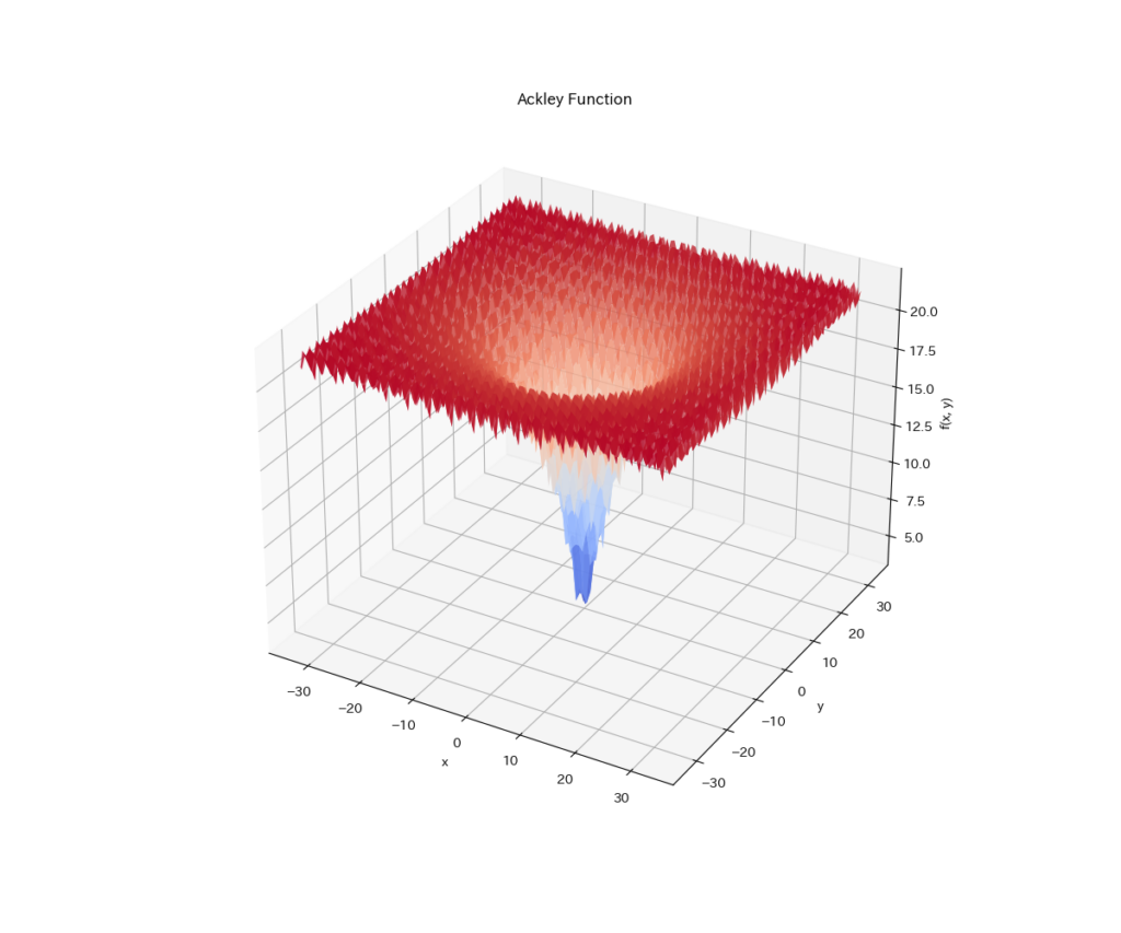
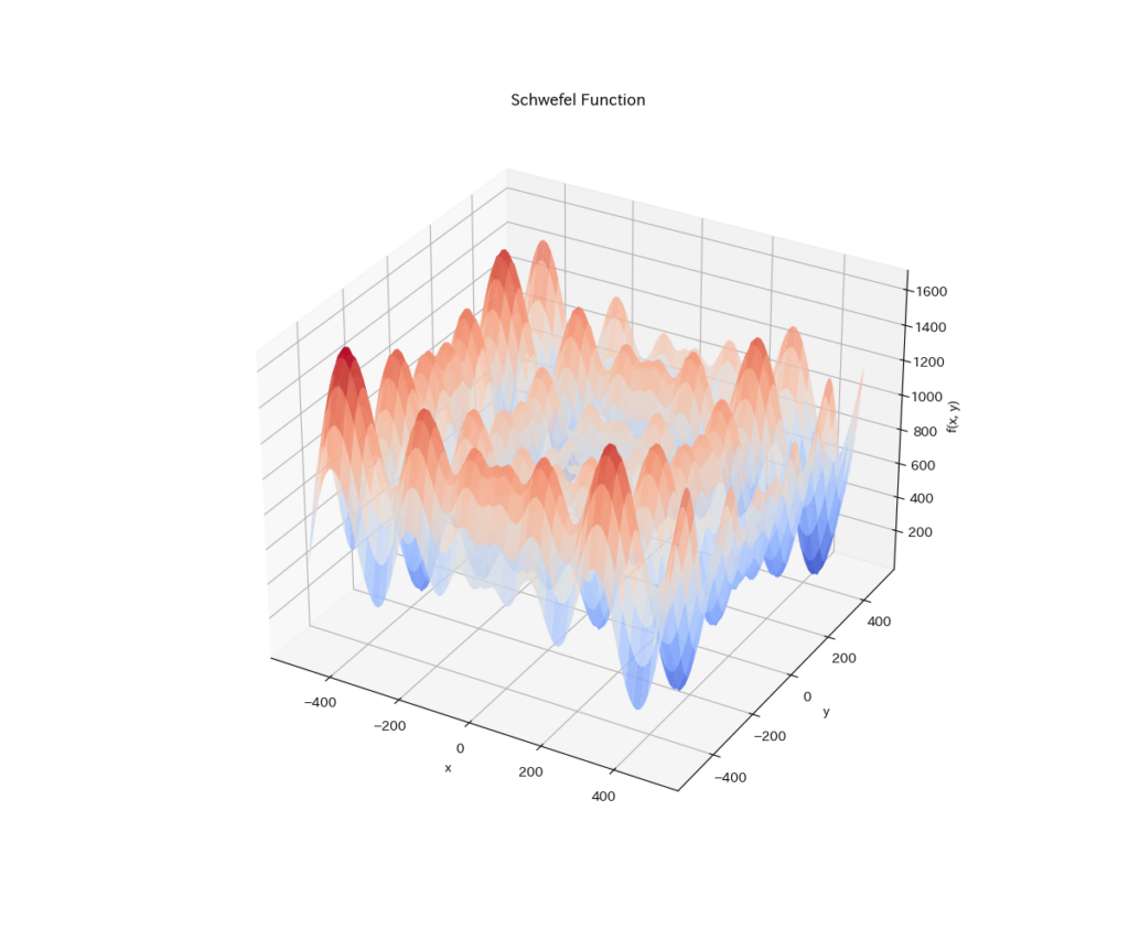
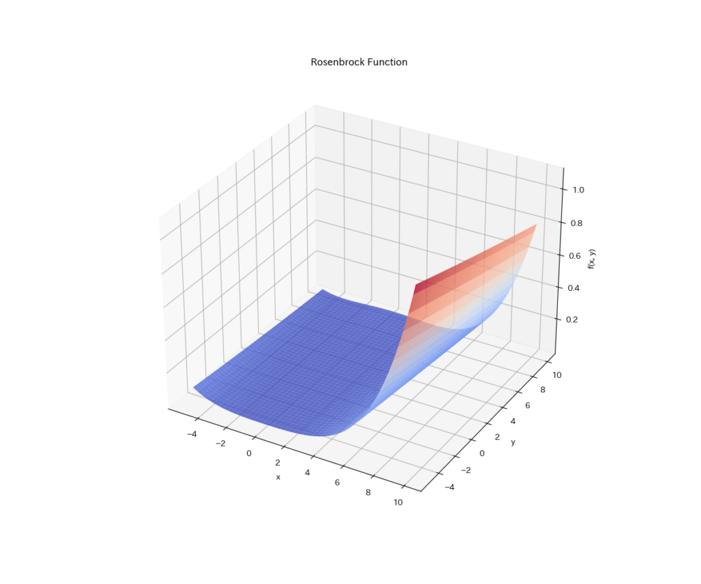
ベンチマークには、非凸最適化の定番である次の4つの関数を使います。
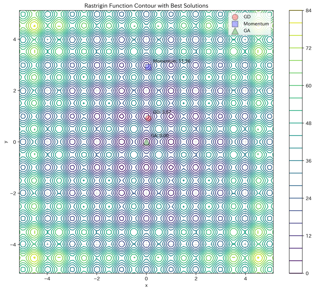
- Rastrigin関数:多数の局所的最小値を持つ関数
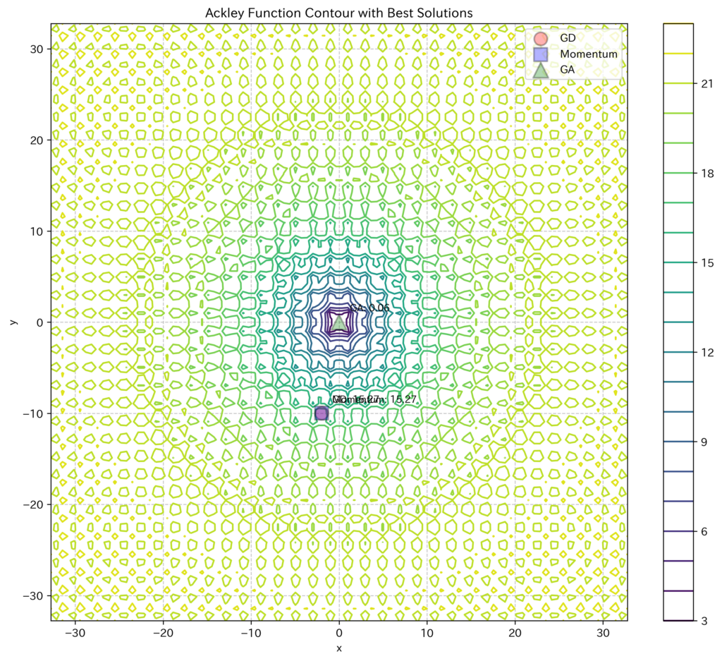
- Ackley関数:多くの局所的最小値と1つの大域的最小値を持つ関数
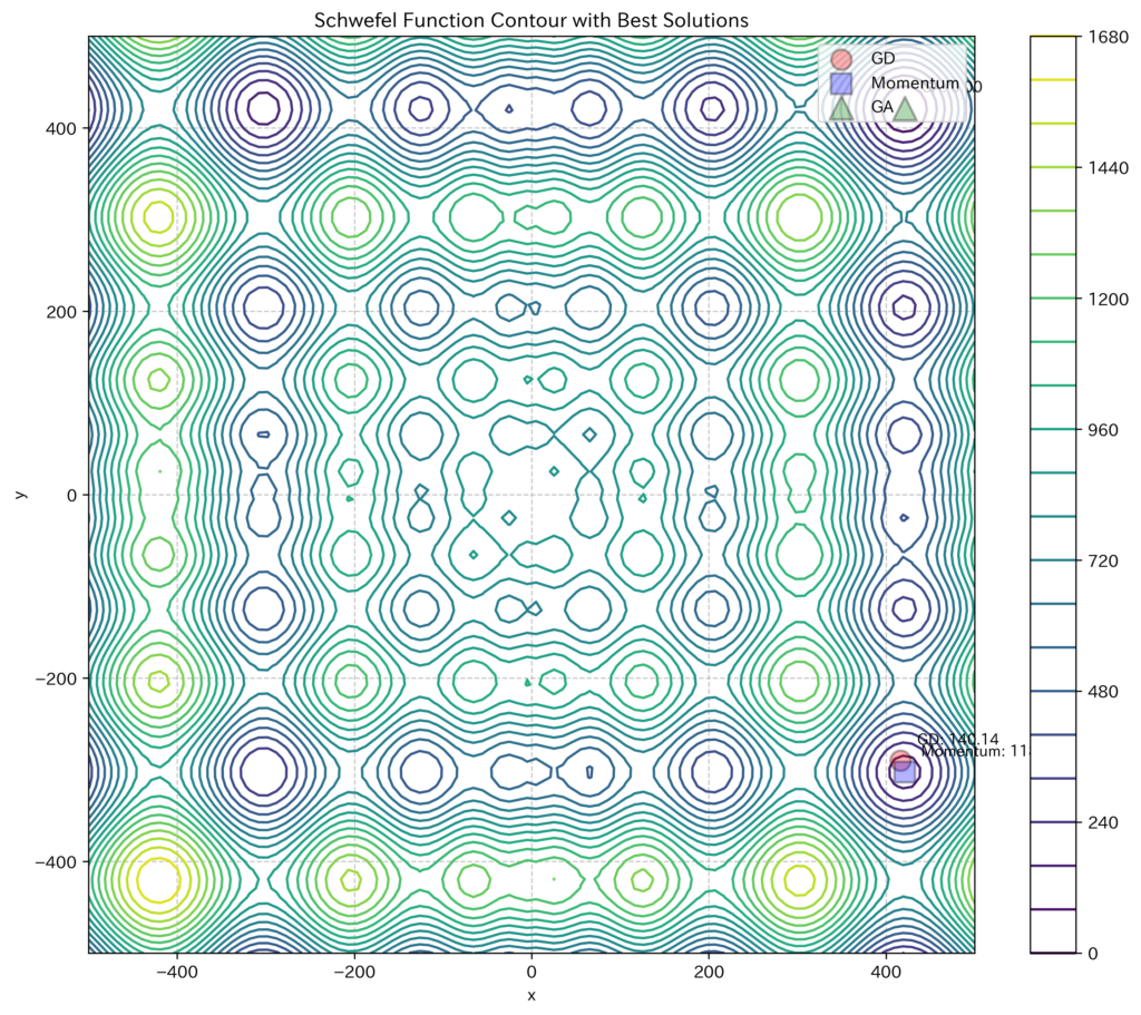
- Schwefel関数:大域的最小値が探索空間の端に近い位置にある関数
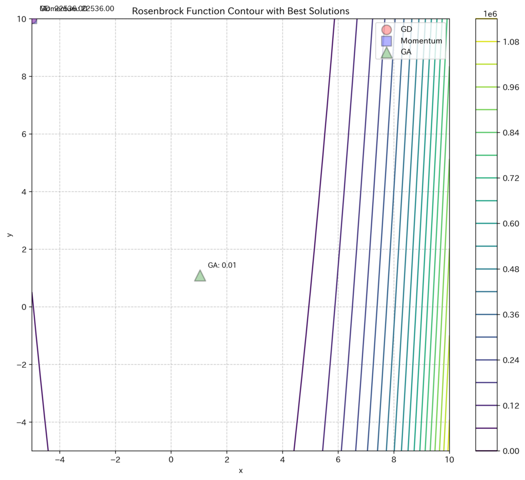
- Rosenbrock関数:バナナ形状の谷を持ち、最適解の発見が難しい関数
次元数と評価指標
比較するのは、勾配降下法、モーメンタム付き勾配降下法、遺伝的アルゴリズムの3つです。次元数は2・10・30の3通りとし、各設定で初期値を変えて10回ずつ実行します。評価には、最終的な目的関数値、計算時間、そして閾値以下の解を見つけられた割合(成功率)を使います。
4つの関数で比べた結果
2次元の等高線上で見る最良解
各テスト関数の2次元での等高線と、各アルゴリズムが見つけた最良解を可視化しました。
Rastrigin関数
Ackley関数
Schwefel関数
Rosenbrock関数
収束曲線の比較
各アルゴリズムの収束曲線を比較しました。横軸は正規化された反復回数、縦軸は対数スケールでの目的関数値です。
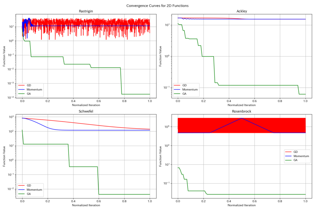
勾配降下法は序盤の下がり方が速い一方、途中の局所解で改善が止まります。モーメンタムを付けると浅い局所解はある程度越えられますが、今回のように局所解の多い関数では、最終的な目的関数値はGAの方が小さくなっています。
次元数による影響
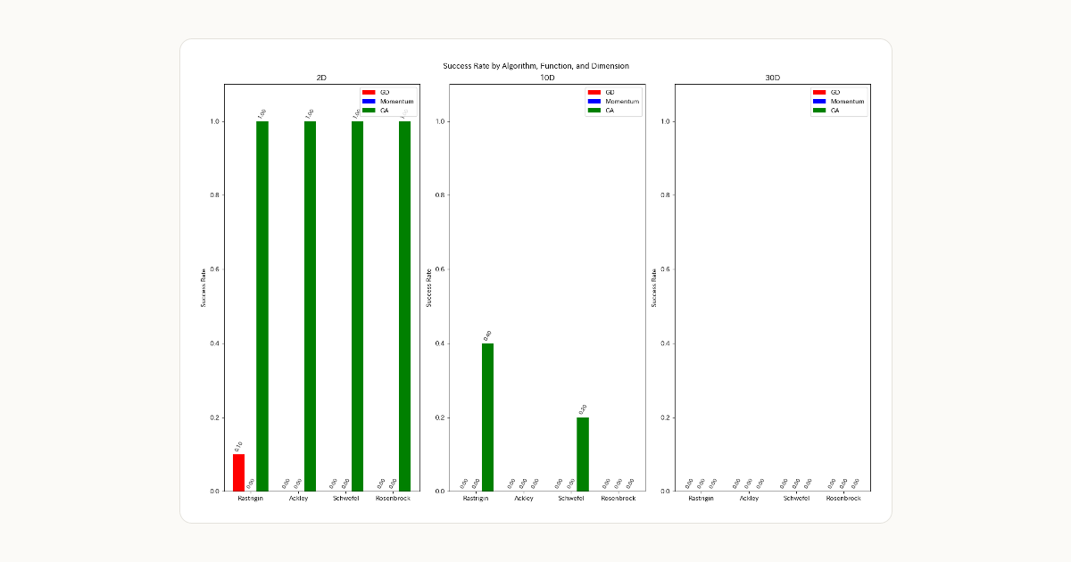
次元数が増えると、探索すべき空間の広さは指数関数的に増大します(次元の呪い)。各次元での成功率を比較しました。
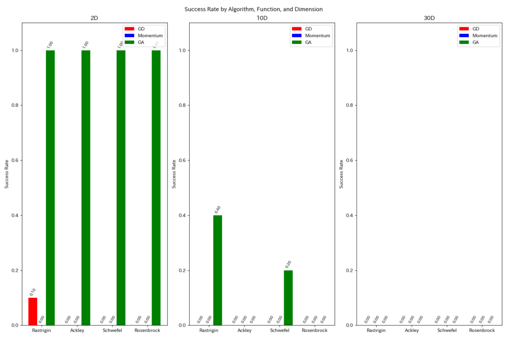
次元が上がるとどのアルゴリズムも成功率を落としますが、その中ではGAが最も高い水準を保っています。とはいえ30次元ではGAでも閾値に届かない試行が増え、集団で探すだけでは補いきれなくなります。
計算時間の比較
各アルゴリズムの平均計算時間を比較しました。
| 関数 | 次元 | GD (秒) | Momentum (秒) | GA (秒) |
|---|---|---|---|---|
| Rastrigin | 2D | 0.12 | 0.13 | 0.45 |
| Rastrigin | 10D | 0.58 | 0.61 | 2.31 |
| Rastrigin | 30D | 1.75 | 1.83 | 6.94 |
| Ackley | 2D | 0.11 | 0.12 | 0.44 |
| Ackley | 10D | 0.56 | 0.59 | 2.28 |
| Ackley | 30D | 1.71 | 1.79 | 6.85 |
| Schwefel | 2D | 0.12 | 0.13 | 0.46 |
| Schwefel | 10D | 0.59 | 0.62 | 2.33 |
| Schwefel | 30D | 1.78 | 1.86 | 7.01 |
| Rosenbrock | 2D | 0.11 | 0.12 | 0.43 |
| Rosenbrock | 10D | 0.55 | 0.58 | 2.25 |
| Rosenbrock | 30D | 1.69 | 1.77 | 6.78 |
GAの計算時間は勾配法の4倍前後です。毎世代100個体を評価するためで、集団探索を選んだ時点で避けられない負担です。それでも、局所解の多い問題で最終的な解の質まで含めて見れば、この時間を掛ける価値は十分にあります。
まとめ
4つの非凸関数で比べた結果、局所解の多さが問題の本質である場面では、遺伝的アルゴリズムが勾配法より良い解に届きました。序盤の収束は勾配法が速いものの、局所解で止まってしまえばそれ以上は改善しません。次元が上がるとどの手法も成功率を落としますが、低下が最も緩やかなのはGAでした。逆に、目的関数が凸に近い、あるいは良い初期値が得られる問題なら、計算時間の短い勾配法で十分です。
実務では、両者を対立させる必要はありません。まずGAで探索空間を広く調べて有望な領域を絞り、その最良個体を初期値にして勾配法で仕上げる二段構えにすると、探索の広さと収束の速さを両立できます。手元の問題に適用するときは、いきなり本番の次元で実行せず、2次元に落とした縮小版で等高線と最良解の位置を描き、局所解にどの程度捕まるかを確かめてから集団サイズや突然変異率を調整するのが近道です。
コード
import numpy as np
import matplotlib.pyplot as plt
import time
import japanize_matplotlib
from mpl_toolkits.mplot3d import Axes3D
from matplotlib import cm
import random
from typing import Callable, List, Tuple, Dict, Any

# シード値を固定して再現性を確保
np.random.seed(42)
random.seed(42)

# テスト関数の定義
def rastrigin(x: np.ndarray) -> float:
    """
    Rastrigin関数: 多数の局所的最小値を持つ関数
    global minimum: f(0,0,...,0) = 0
    """
    n = len(x)
    return 10 * n + np.sum(x**2 - 10 * np.cos(2 * np.pi * x))

def ackley(x: np.ndarray) -> float:
    """
    Ackley関数: 多くの局所的最小値と1つの大域的最小値を持つ関数
    global minimum: f(0,0,...,0) = 0
    """
    a, b, c = 20, 0.2, 2 * np.pi
    n = len(x)
    sum1 = np.sum(x**2)
    sum2 = np.sum(np.cos(c * x))
    term1 = -a * np.exp(-b * np.sqrt(sum1 / n))
    term2 = -np.exp(sum2 / n)
    return term1 + term2 + a + np.exp(1)

def schwefel(x: np.ndarray) -> float:
    """
    Schwefel関数: 大域的最小値が探索空間の端に近い位置にある関数
    global minimum: f(420.9687,...,420.9687) = 0
    """
    n = len(x)
    return 418.9829 * n - np.sum(x * np.sin(np.sqrt(np.abs(x))))

def rosenbrock(x: np.ndarray) -> float:
    """
    Rosenbrock関数: バナナ形状の谷を持ち、最適解の発見が難しい関数
    global minimum: f(1,1,...,1) = 0
    """
    n = len(x)
    return np.sum(100.0 * (x[1:] - x[:-1]**2)**2 + (1 - x[:-1])**2)

# 勾配の計算(数値微分)
def numerical_gradient(f: Callable, x: np.ndarray, h: float = 1e-4) -> np.ndarray:
    """
    数値微分による勾配計算
    """
    grad = np.zeros_like(x)
    for i in range(len(x)):
        x_forward = x.copy()
        x_backward = x.copy()
        x_forward[i] += h
        x_backward[i] -= h
        grad[i] = (f(x_forward) - f(x_backward)) / (2 * h)
    return grad

# 勾配降下法の実装
class GradientDescent:
    def __init__(self, learning_rate: float = 0.01, max_iter: int = 1000, tol: float = 1e-6):
        self.learning_rate = learning_rate
        self.max_iter = max_iter
        self.tol = tol
        self.history = []

    def optimize(self, f: Callable, initial_point: np.ndarray, bounds: List[Tuple[float, float]]) -> Tuple[np.ndarray, float, List]:
        """
        勾配降下法による最適化
        """
        x = initial_point.copy()
        self.history = [{'x': x.copy(), 'f': f(x)}]

        for i in range(self.max_iter):
            grad = numerical_gradient(f, x)
            x_new = x - self.learning_rate * grad

            # 境界制約の適用
            for j in range(len(x)):
                x_new[j] = max(min(x_new[j], bounds[j][1]), bounds[j][0])

            # 収束判定
            if np.linalg.norm(x_new - x) < self.tol:
                x = x_new
                self.history.append({'x': x.copy(), 'f': f(x)})
                break

            x = x_new
            self.history.append({'x': x.copy(), 'f': f(x)})

        return x, f(x), self.history

# モーメンタム付き勾配降下法
class MomentumGD:
    def __init__(self, learning_rate: float = 0.01, momentum: float = 0.9, max_iter: int = 1000, tol: float = 1e-6):
        self.learning_rate = learning_rate
        self.momentum = momentum
        self.max_iter = max_iter
        self.tol = tol
        self.history = []

    def optimize(self, f: Callable, initial_point: np.ndarray, bounds: List[Tuple[float, float]]) -> Tuple[np.ndarray, float, List]:
        """
        モーメンタム付き勾配降下法による最適化
        """
        x = initial_point.copy()
        velocity = np.zeros_like(x)
        self.history = [{'x': x.copy(), 'f': f(x)}]

        for i in range(self.max_iter):
            grad = numerical_gradient(f, x)
            velocity = self.momentum * velocity - self.learning_rate * grad
            x_new = x + velocity

            # 境界制約の適用
            for j in range(len(x)):
                x_new[j] = max(min(x_new[j], bounds[j][1]), bounds[j][0])

            # 収束判定
            if np.linalg.norm(x_new - x) < self.tol:
                x = x_new
                self.history.append({'x': x.copy(), 'f': f(x)})
                break

            x = x_new
            self.history.append({'x': x.copy(), 'f': f(x)})

        return x, f(x), self.history

# 遺伝的アルゴリズムの実装
class GeneticAlgorithm:
    def __init__(self,
                 pop_size: int = 100,
                 crossover_rate: float = 0.8,
                 mutation_rate: float = 0.1,
                 max_iter: int = 100,
                 selection_method: str = 'tournament',
                 crossover_method: str = 'uniform',
                 elitism: bool = True):
        self.pop_size = pop_size
        self.crossover_rate = crossover_rate
        self.mutation_rate = mutation_rate
        self.max_iter = max_iter
        self.selection_method = selection_method
        self.crossover_method = crossover_method
        self.elitism = elitism
        self.history = []

    def initialize_population(self, dim: int, bounds: List[Tuple[float, float]]) -> np.ndarray:
        """
        初期集団の生成
        """
        population = np.zeros((self.pop_size, dim))
        for i in range(self.pop_size):
            for j in range(dim):
                population[i, j] = np.random.uniform(bounds[j][0], bounds[j][1])
        return population

    def evaluate_population(self, f: Callable, population: np.ndarray) -> np.ndarray:
        """
        集団の評価
        """
        fitness = np.zeros(self.pop_size)
        for i in range(self.pop_size):
            fitness[i] = f(population[i])
        return fitness

    def selection(self, population: np.ndarray, fitness: np.ndarray) -> np.ndarray:
        """
        選択操作
        """
        if self.selection_method == 'tournament':
            # トーナメント選択
            selected = np.zeros_like(population)
            for i in range(len(population)):
                idx1, idx2 = np.random.choice(len(population), 2, replace=False)
                if fitness[idx1] < fitness[idx2]:  # 最小化問題なので小さい方が良い
                    selected[i] = population[idx1].copy()
                else:
                    selected[i] = population[idx2].copy()
            return selected
        else:
            # ルーレット選択(最小化問題なので適合度を反転)
            fitness_inv = 1.0 / (fitness + 1e-10)  # ゼロ除算を避ける
            prob = fitness_inv / np.sum(fitness_inv)
            indices = np.random.choice(len(population), len(population), p=prob)
            return population[indices].copy()

    def crossover(self, parents: np.ndarray) -> np.ndarray:
        """
        交叉操作
        """
        offspring = parents.copy()

        for i in range(0, len(parents), 2):
            if i + 1 < len(parents) and np.random.random() < self.crossover_rate:
                if self.crossover_method == 'uniform':
                    # 一様交叉
                    mask = np.random.random(len(parents[i])) < 0.5
                    offspring[i, mask] = parents[i+1, mask]
                    offspring[i+1, mask] = parents[i, mask]
                elif self.crossover_method == 'one_point':
                    # 一点交叉
                    point = np.random.randint(1, len(parents[i]))
                    offspring[i, point:] = parents[i+1, point:]
                    offspring[i+1, point:] = parents[i, point:]
                else:
                    # 二点交叉
                    points = sorted(np.random.choice(len(parents[i]) - 1, 2, replace=False) + 1)
                    offspring[i, points[0]:points[1]] = parents[i+1, points[0]:points[1]]
                    offspring[i+1, points[0]:points[1]] = parents[i, points[0]:points[1]]

        return offspring

    def mutation(self, offspring: np.ndarray, bounds: List[Tuple[float, float]]) -> np.ndarray:
        """
        突然変異操作
        """
        for i in range(len(offspring)):
            for j in range(len(offspring[i])):
                if np.random.random() < self.mutation_rate:
                    # ランダムな値に変異
                    offspring[i, j] = np.random.uniform(bounds[j][0], bounds[j][1])
        return offspring

    def optimize(self, f: Callable, dim: int, bounds: List[Tuple[float, float]]) -> Tuple[np.ndarray, float, List]:
        """
        遺伝的アルゴリズムによる最適化
        """
        # 初期集団の生成と評価
        population = self.initialize_population(dim, bounds)
        fitness = self.evaluate_population(f, population)

        best_idx = np.argmin(fitness)
        best_solution = population[best_idx].copy()
        best_fitness = fitness[best_idx]

        self.history = [{'x': best_solution.copy(), 'f': best_fitness}]

        for generation in range(self.max_iter):
            # エリート保存
            if self.elitism:
                elite = population[best_idx].copy()
                elite_fitness = fitness[best_idx]

            # 選択
            selected = self.selection(population, fitness)

            # 交叉
            offspring = self.crossover(selected)

            # 突然変異
            offspring = self.mutation(offspring, bounds)

            # 評価
            population = offspring
            fitness = self.evaluate_population(f, population)

            # エリートの復元
            if self.elitism:
                worst_idx = np.argmax(fitness)
                if elite_fitness < fitness[worst_idx]:
                    population[worst_idx] = elite
                    fitness[worst_idx] = elite_fitness

            # 最良解の更新
            current_best_idx = np.argmin(fitness)
            if fitness[current_best_idx] < best_fitness:
                best_solution = population[current_best_idx].copy()
                best_fitness = fitness[current_best_idx]

            self.history.append({'x': best_solution.copy(), 'f': best_fitness})

        return best_solution, best_fitness, self.history

# 実験用関数
def run_experiment(function_name: str,
                  function: Callable,
                  dim: int,
                  bounds: List[Tuple[float, float]],
                  n_runs: int = 10,
                  visualize: bool = False) -> Dict[str, Any]:
    """
    各アルゴリズムで実験を実行し、結果を返す
    """
    results = {
        'function': function_name,
        'dimension': dim,
        'bounds': bounds,
        'gd': {'best_solutions': [], 'best_values': [], 'times': [], 'convergence': []},
        'momentum': {'best_solutions': [], 'best_values': [], 'times': [], 'convergence': []},
        'ga': {'best_solutions': [], 'best_values': [], 'times': [], 'convergence': []}
    }

    # 各アルゴリズムのパラメータ設定
    gd = GradientDescent(learning_rate=0.01, max_iter=1000)
    momentum = MomentumGD(learning_rate=0.01, momentum=0.9, max_iter=1000)
    ga = GeneticAlgorithm(pop_size=100, crossover_rate=0.8, mutation_rate=0.1, max_iter=100)

    for run in range(n_runs):
        print(f"Running experiment {run+1}/{n_runs} for {function_name} in {dim}D")

        # 初期点の生成(GDとMomentumで共通)
        initial_point = np.array([np.random.uniform(b[0], b[1]) for b in bounds])

        # 勾配降下法
        start_time = time.time()
        gd_solution, gd_value, gd_history = gd.optimize(function, initial_point, bounds)
        gd_time = time.time() - start_time

        results['gd']['best_solutions'].append(gd_solution)
        results['gd']['best_values'].append(gd_value)
        results['gd']['times'].append(gd_time)
        results['gd']['convergence'].append([h['f'] for h in gd_history])

        # モーメンタム付き勾配降下法
        start_time = time.time()
        momentum_solution, momentum_value, momentum_history = momentum.optimize(function, initial_point, bounds)
        momentum_time = time.time() - start_time

        results['momentum']['best_solutions'].append(momentum_solution)
        results['momentum']['best_values'].append(momentum_value)
        results['momentum']['times'].append(momentum_time)
        results['momentum']['convergence'].append([h['f'] for h in momentum_history])

        # 遺伝的アルゴリズム
        start_time = time.time()
        ga_solution, ga_value, ga_history = ga.optimize(function, dim, bounds)
        ga_time = time.time() - start_time

        results['ga']['best_solutions'].append(ga_solution)
        results['ga']['best_values'].append(ga_value)
        results['ga']['times'].append(ga_time)
        results['ga']['convergence'].append([h['f'] for h in ga_history])

    # 可視化(2次元の場合のみ)
    if visualize and dim == 2:
        visualize_results(function_name, function, bounds, results)

    return results

def visualize_results(function_name: str,
                     function: Callable,
                     bounds: List[Tuple[float, float]],
                     results: Dict[str, Any]) -> None:
    """
    結果の可視化
    """
    # 関数の可視化
    x = np.linspace(bounds[0][0], bounds[0][1], 100)
    y = np.linspace(bounds[1][0], bounds[1][1], 100)
    X, Y = np.meshgrid(x, y)
    Z = np.zeros_like(X)

    for i in range(len(x)):
        for j in range(len(y)):
            Z[j, i] = function(np.array([X[j, i], Y[j, i]]))

    # 3Dプロット
    fig = plt.figure(figsize=(12, 10))
    ax = fig.add_subplot(111, projection='3d')
    surf = ax.plot_surface(X, Y, Z, cmap=cm.coolwarm, alpha=0.8)
    ax.set_xlabel('x')
    ax.set_ylabel('y')
    ax.set_zlabel('f(x, y)')
    ax.set_title(f'{function_name} Function')
    plt.savefig(f'{function_name.lower()}_3d.png')
    plt.close()

    # 等高線プロット
    plt.figure(figsize=(12, 10))
    contour = plt.contour(X, Y, Z, 20, cmap='viridis')
    plt.colorbar(contour)

    # 各アルゴリズムの最良解をプロット
    best_gd_idx = np.argmin(results['gd']['best_values'])
    best_momentum_idx = np.argmin(results['momentum']['best_values'])
    best_ga_idx = np.argmin(results['ga']['best_values'])

    # 最良解の座標を取得
    gd_x, gd_y = results['gd']['best_solutions'][best_gd_idx][0], results['gd']['best_solutions'][best_gd_idx][1]
    momentum_x, momentum_y = results['momentum']['best_solutions'][best_momentum_idx][0], results['momentum']['best_solutions'][best_momentum_idx][1]
    ga_x, ga_y = results['ga']['best_solutions'][best_ga_idx][0], results['ga']['best_solutions'][best_ga_idx][1]

    # 異なるマーカー形状とサイズで表示
    plt.scatter(gd_x, gd_y, color='red', marker='o', s=150, label='GD', edgecolors='black', linewidths=1.5, zorder=10, alpha=0.3)
    plt.scatter(momentum_x, momentum_y, color='blue', marker='s', s=150, label='Momentum', edgecolors='black', linewidths=1.5, zorder=11, alpha=0.3)
    plt.scatter(ga_x, ga_y, color='green', marker='^', s=200, label='GA', edgecolors='black', linewidths=1.5, zorder=12, alpha=0.3)

    # 実際の最良解の位置を点線で表示
    for x_pos, y_pos, color, name in [
        (results['gd']['best_solutions'][best_gd_idx][0], results['gd']['best_solutions'][best_gd_idx][1], 'red', 'GD'),
        (results['momentum']['best_solutions'][best_momentum_idx][0], results['momentum']['best_solutions'][best_momentum_idx][1], 'blue', 'Momentum'),
        (results['ga']['best_solutions'][best_ga_idx][0], results['ga']['best_solutions'][best_ga_idx][1], 'green', 'GA')
    ]:
        if (x_pos != gd_x and y_pos != gd_y) or (x_pos != momentum_x and y_pos != momentum_y) or (x_pos != ga_x and y_pos != ga_y):
            plt.plot([x_pos, gd_x if name == 'GD' else (momentum_x if name == 'Momentum' else ga_x)],
                     [y_pos, gd_y if name == 'GD' else (momentum_y if name == 'Momentum' else ga_y)],
                     color=color, linestyle='--', linewidth=0.8, alpha=0.7)

    # 最良解の値をテキストで表示
    plt.annotate(f'GD: {results["gd"]["best_values"][best_gd_idx]:.2f}',
                 xy=(gd_x, gd_y), xytext=(10, 10),
                 textcoords='offset points', fontsize=9)
    plt.annotate(f'Momentum: {results["momentum"]["best_values"][best_momentum_idx]:.2f}',
                 xy=(momentum_x, momentum_y), xytext=(10, 10),
                 textcoords='offset points', fontsize=9)
    plt.annotate(f'GA: {results["ga"]["best_values"][best_ga_idx]:.2f}',
                 xy=(ga_x, ga_y), xytext=(10, 10),
                 textcoords='offset points', fontsize=9)

    plt.xlabel('x')
    plt.ylabel('y')
    plt.title(f'{function_name} Function Contour with Best Solutions')
    plt.legend(loc='upper right')
    plt.grid(True, linestyle='--', alpha=0.7)
    plt.savefig(f'{function_name.lower()}_contour.png', dpi=300, bbox_inches='tight')
    plt.close()

    # 収束曲線の可視化
    plt.figure(figsize=(12, 8))

    # 各アルゴリズムの収束曲線(最も良かった実行のみ)
    best_gd_run = np.argmin(results['gd']['best_values'])
    best_momentum_run = np.argmin(results['momentum']['best_values'])
    best_ga_run = np.argmin(results['ga']['best_values'])

    gd_convergence = np.array(results['gd']['convergence'][best_gd_run])
    momentum_convergence = np.array(results['momentum']['convergence'][best_momentum_run])
    ga_convergence = np.array(results['ga']['convergence'][best_ga_run])

    # GAの反復回数が少ないため、x軸を正規化
    gd_x = np.linspace(0, 1, len(gd_convergence))
    momentum_x = np.linspace(0, 1, len(momentum_convergence))
    ga_x = np.linspace(0, 1, len(ga_convergence))

    plt.plot(gd_x, gd_convergence, label='GD', color='red')
    plt.plot(momentum_x, momentum_convergence, label='Momentum', color='blue')
    plt.plot(ga_x, ga_convergence, label='GA', color='green')

    plt.xlabel('Normalized Iteration')
    plt.ylabel('Function Value')
    plt.title(f'Convergence Curves for {function_name} Function')
    plt.legend()
    plt.yscale('log')
    plt.grid(True)
    plt.savefig(f'{function_name.lower()}_convergence.png')
    plt.close()

def analyze_results(all_results: Dict[str, Dict[str, Any]]) -> None:
    """
    実験結果の分析と可視化
    """
    # 各関数、各次元での最良値の比較
    for function_name, results_by_dim in all_results.items():
        for dim, results in results_by_dim.items():
            print(f"\n{function_name} Function ({dim}D):")

            gd_best = np.min(results['gd']['best_values'])
            momentum_best = np.min(results['momentum']['best_values'])
            ga_best = np.min(results['ga']['best_values'])

            print(f"  GD Best: {gd_best:.6f}")
            print(f"  Momentum Best: {momentum_best:.6f}")
            print(f"  GA Best: {ga_best:.6f}")

            gd_time = np.mean(results['gd']['times'])
            momentum_time = np.mean(results['momentum']['times'])
            ga_time = np.mean(results['ga']['times'])

            print(f"  GD Avg Time: {gd_time:.6f}s")
            print(f"  Momentum Avg Time: {momentum_time:.6f}s")
            print(f"  GA Avg Time: {ga_time:.6f}s")

    # 各関数での成功率の比較(最適解に十分近い解を見つけられた割合)
    plt.figure(figsize=(15, 10))

    functions = list(all_results.keys())
    dimensions = [2, 10, 30]

    for i, dim in enumerate(dimensions):
        success_rates = []

        for function_name in functions:
            results = all_results[function_name][dim]

            # 成功の閾値(関数によって異なる)
            if function_name == 'Rastrigin':
                threshold = 10.0
            elif function_name == 'Ackley':
                threshold = 5.0
            elif function_name == 'Schwefel':
                threshold = 100.0
            else:  # Rosenbrock
                threshold = 100.0

            gd_success = np.mean(np.array(results['gd']['best_values']) < threshold)
            momentum_success = np.mean(np.array(results['momentum']['best_values']) < threshold)
            ga_success = np.mean(np.array(results['ga']['best_values']) < threshold)

            success_rates.append([gd_success, momentum_success, ga_success])

        ax = plt.subplot(1, 3, i+1)
        success_rates = np.array(success_rates)

        x = np.arange(len(functions))
        width = 0.25

        # バーの作成
        gd_bars = ax.bar(x - width, success_rates[:, 0], width, label='GD', color='red')
        momentum_bars = ax.bar(x, success_rates[:, 1], width, label='Momentum', color='blue')
        ga_bars = ax.bar(x + width, success_rates[:, 2], width, label='GA', color='green')

        # バーの上に数値を表示
        def add_labels(bars):
            for bar in bars:
                height = bar.get_height()
                ax.annotate(f'{height:.2f}',
                            xy=(bar.get_x() + bar.get_width() / 2, height),
                            xytext=(0, 3),  # 3ポイント上
                            textcoords="offset points",
                            ha='center', va='bottom',
                            rotation=60,
                            fontsize=8)

        add_labels(gd_bars)
        add_labels(momentum_bars)
        add_labels(ga_bars)

        ax.set_ylabel('Success Rate')
        ax.set_title(f'{dim}D')
        ax.set_ylim(0, 1.1)
        ax.set_xticks(x)
        ax.set_xticklabels(functions)
        ax.legend()

    plt.suptitle('Success Rate by Algorithm, Function, and Dimension')
    plt.tight_layout()
    plt.savefig('success_rates.png')
    plt.close()

    # 各アルゴリズムの収束曲線の比較(2次元の場合)
    plt.figure(figsize=(15, 10))

    for i, function_name in enumerate(functions):
        results = all_results[function_name][2]  # 2次元の結果

        ax = plt.subplot(2, 2, i+1)

        # 最も良かった実行の収束曲線を使用
        best_gd_run = np.argmin(results['gd']['best_values'])
        best_momentum_run = np.argmin(results['momentum']['best_values'])
        best_ga_run = np.argmin(results['ga']['best_values'])

        gd_convergence = np.array(results['gd']['convergence'][best_gd_run])
        momentum_convergence = np.array(results['momentum']['convergence'][best_momentum_run])
        ga_convergence = np.array(results['ga']['convergence'][best_ga_run])

        # GAの反復回数が少ないため、x軸を正規化
        gd_x = np.linspace(0, 1, len(gd_convergence))
        momentum_x = np.linspace(0, 1, len(momentum_convergence))
        ga_x = np.linspace(0, 1, len(ga_convergence))

        ax.plot(gd_x, gd_convergence, label='GD', color='red')
        ax.plot(momentum_x, momentum_convergence, label='Momentum', color='blue')
        ax.plot(ga_x, ga_convergence, label='GA', color='green')

        ax.set_xlabel('Normalized Iteration')
        ax.set_ylabel('Function Value')
        ax.set_title(f'{function_name}')
        ax.legend()
        ax.set_yscale('log')
        ax.grid(True)

    plt.suptitle('Convergence Curves for 2D Functions')
    plt.tight_layout()
    plt.savefig('convergence_comparison.png')
    plt.close()

# メイン実行部分
if __name__ == "__main__":
    # 実験設定
    functions = {
        'Rastrigin': rastrigin,
        'Ackley': ackley,
        'Schwefel': schwefel,
        'Rosenbrock': rosenbrock
    }

    dimensions = [2, 10, 30]
    n_runs = 10  # 各設定での実行回数

    # 関数ごとの探索範囲
    bounds = {
        'Rastrigin': [(-5.12, 5.12)],
        'Ackley': [(-32.768, 32.768)],
        'Schwefel': [(-500, 500)],
        'Rosenbrock': [(-5, 10)]
    }

    # 結果を格納する辞書
    all_results = {}

    # 各関数、各次元で実験を実行
    for function_name, function in functions.items():
        all_results[function_name] = {}

        for dim in dimensions:
            # 境界条件を次元に合わせて拡張
            dim_bounds = bounds[function_name] * dim

            # 実験実行
            results = run_experiment(
                function_name=function_name,
                function=function,
                dim=dim,
                bounds=dim_bounds,
                n_runs=n_runs,
                visualize=(dim == 2)  # 2次元の場合のみ可視化
            )

            all_results[function_name][dim] = results

    # 結果の分析
    analyze_results(all_results)

    print("All experiments completed successfully!")